Artificial Intelligence
UNIT – I
Part-2
1.2.7
Problems, Problem Spaces, and Search
In the last section, we had a brief description of the kinds of
problems with which Al is typically concerned, as well as a couple of examples
of the techniques it offers to solve those problems. To build a system to solve
a particular problem, we need to do four things:
- Define the problem precisely. This
definition must include precise specifications of what the initial situation(s)
will be as well as what final situations constitute acceptable solutions
to the problem.
- Analyze the problem. A few very
important features can have an immense impact on the appropriateness of
various possible techniques for solving the problem.
- Isolate and represent the task
knowledge that is necessary to solve the problem.
- Choose the best problem-solving
technique(s) and apply it (them) to the particular problem.
Defining the Problem as a State Space Search
A Water Jug Problem: You
are given two jugs, a 4-gallon one and a 3-gallon one. Neither has any
measuring markers on it. There is a pump, that can be used to fill the jugs
with water. How can you get exactly 2 gallons of water into the 4-gallon jug?
The state space for this problem can be described as the set of
ordered pairs of integers (x, y), such that x =0, 1,2,3, or 4 and y =0, 1, 2,
or 3; x represents the number of gallons of water in the 4-gallon jug, and y
represents the quantity of water in the 3-gallon jug. The start state is (0, 0).
The goal state is (2, n) for any
value of n (since the problem does
not specify how many gallons need to be in the 3-gallon jug).
The operators to be used to solve the problem can be described as
shown in Figure 1.2. As in the chess problem, they are represented as rules
whose left sides are matched against the current state and whose right sides
describe the new state that results from applying the rule. Notice that in
order to describe the operators completely, it was necessary to make explicit
some assumptions not mentioned in the problem statement. We have assumed that
we can fill a jug from the pump, that we can pour water out of a jug onto the
ground, that we can pour water from one jug to another, and that there are no
other measuring devices available. Additional assumptions such as these are
almost always required when converting from a typical problem statement given
in English to a formal representation of the problem suitable for use by a
program.
1
(x ,y) →
(4, y) Fill the 4-gallon jug.
if x < 4
2 (x, y) →
(x, 3) Fill the 3 – gallon jug.
if y <3
if y <3
3
(x, y) → (x
- d, y) Pour some
water out of
if x > 0 the 4 – gallon jug
4
(x, y) → (x,
y - d) Pour some
water out of
if y > 0 the 3 – gallon jug
5 (x, y) →
(0, y) Empty the 4-gallon jug
if x > 0 on the ground
6
(x, y) → (x,
0) Empty the
3-gallon jug
if y > 0 on the ground
7 (x, y) →
(4, y – (4 – x)) Pour water from
the
if x+ y ≥ 4 and y > 0 3-gallon jug into the
4-gallon jug until the
4-gallon jug is full
4-gallon jug until the
4-gallon jug is full
if x+ y ≥ 3 and x > 0 4-gallon jug into the
3-gallon jug until tile
3-gallon jug is full
3-gallon jug until tile
3-gallon jug is full
9 (x, y) →
(x + y, 0) Pour all
the water
from the 3-gallon 4ug
into the 4-gallon jug
from the 3-gallon 4ug
into the 4-gallon jug
10 (x, y) →
(0, x + y) Pour all the water
from the 4-gallon jug
into the 3-gallon jug
from the 4-gallon jug
into the 3-gallon jug
11 (0, 2) → (2,0) Pour
the 2 gallons
from the 3-gallon jug
into the 4-gallon jug
from the 3-gallon jug
into the 4-gallon jug
12 (2, y) →
(0, y) Empty the 2 gallons in
the 4-gallon jug on
the ground
the 4-gallon jug on
the ground
Figure 1.2:
Production Rules for the Water Jug Problem
To solve the water jug problem, all we need, in addition to the
problem description given above, is a control structure that loops through a
simple cycle in which some rule whose left side matches the current state is
chosen, the appropriate change to the state is made as described in the
corresponding right side, and the resulting state is checked to see if it
corresponds to a goal state. As long as it does not, the cycle continues.
Clearly the speed with which the problem gets solved depends on the mechanism
that is used to select the next operation to be performed.
For the water jug problem, as with many others, there are several
sequences of operators that solve the problem. One such sequence is shown in
Figure 1.3. Often, a problem contains the explicit or implied statement that
the shortest (or cheapest) such sequence be found. If present, this requirement
will have a significant effect on the choice of an appropriate mechanism to
guide the search for a solution.
Several
issues that often arise in converting an informal problem statement into a
formal problem description are illustrated by this sample water jug problem.
The first of these issues concerns the role of the conditions that occur in the
left sides, of the rules. All but one of the rules shown in Figure 1.2 contains
conditions that must be satisfied before the operator described by the rule can
be applied. For example, the first rule says, “If the 4-gallon jug is not
already full, fill it.” This rule could, however, have been written as, “Fill
the 4-gallon jug,” since it is physically possible to fill the jug even if it
is already full. It is stupid to do so since no change in the problem state
results, but it is possible. By encoding in the left sides of the rules
constraints that are not strictly necessary but that restrict the application
of the rules to states in which the rules are most likely to lead to a
solution, we can generally increase the efficiency of the problem-solving
program that uses the rules.
Gallons in the Gallons in the Rules Applied
4-Gallon Jug 3-Gallon Jug
4-Gallon Jug 3-Gallon Jug
0 0
2
0
3
9
3
0
2
3 3
7
4
2
5 or 12
0
2
9 or 11
2 0
Figure 1.3: One Solution to the Water Jug Problem
Each entry in the move vector corresponds to a rule that describes
an operation. The left side of each rule describes a board configuration and is
represented implicitly by the index position. The right side of each rule
describes the operation to be performed and is represented by a nine-element vector
that corresponds to the resulting board configuration. Each of these rules is
maximally specific; it applies only to a single board configuration, and, as a
result, no search is required when such rules are used. However, the drawback
to this extreme approach is that the problem solver can take no action at all
in a novel situation. In fact, essentially no problem solving ever really
occurs. For a tic-tac-toe playing program, this is not a serious problem, since
it k possible to enumerate all the situations (i.e., board configurations) that
may occur. But for most problems, this is not the case. In order to solve new
problems, more general rules must be available.
A second issue is exemplified by rules 3 and 4 in Figure 1.2. Should
they or should they not be included in the list of available operators?
Emptying an unmeasured amount of water onto the ground is certainly allowed by
the problem statement. But a superficial preliminary analysis of the problem
makes it clear that doing so will never get us any closer to a solution. Again,
we see the tradeoff between writing a set of rules that describe just the
problem itself, as opposed to a set of rules that describe both the problem and
some knowledge about its solution.
Rules 11 and 12 illustrate a third issue. To see the problem-solving
knowledge that these rules represent, look at the last two steps of the
solution shown in Figure 1.3. Once the state (4, 2)is reached, it is obvious
what to do next. The desired 2 gallons have been produced, but they are in the
wrong jug. So the thing to do is to move them (rule 11). But before that can be
done, the water that is already in the 4-gallon jug must be emptied out (rule
12). The idea behind these special-purpose rules is to capture the special-case
knowledge that can be used at this stage in solving the problem. These rules do
not actually add power to the system since the operations they describe are
already provided by rule 9 (in the case of rule 11) and by rule 5 (in the case
of rule 12). In fact, depending on the control strategy that is used for
selecting rules to use during problem solving, the use of these rules may
degrade performance. But the use of these rules may also improve performance if
preference is given to special-case rules.
The first step toward the design of a program to solve a problem
must be the creation of a formal and manipulable description of the problem
itself. Ultimately, we would like to be able to write program that can
themselves produce such formal descriptions from informal ones. This process is
called operationalization. The problems are artificial and highly structured.
For other problems, particularly naturally occurring ones, this step is much
more difficult. Consider, for example, the task of specifying precisely what it
means to understand an English sentence. Although such a specification must
somehow be provided before we can design a program to solve the problem,
producing such a specification is itself a very hard problem. Although our
ultimate goal is to be able to solve difficult, unstructured problems, such as
natural language understanding, it is useful to explore simpler problems, such
as the water jug problem, in order to gain insight into the details of methods
that can form the basis for solutions to the harder problems.
In order
to provide a formal description of a problem, we must do the following:
- Define a state space that contains
all the possible configurations of the relevant objects (and perhaps some
impossible ones). It is, of course, possible to define this space without
explicitly enumerating all of the states it contains.
- Specify one or more states within
that space that describe possible situations from
which the problem-solving process may start. These states are called the initial states.
- Specify one or more states that
would be acceptable as solutions to the problem. These states are called
goal states.
- Specify a set of rules that describe the actions (operators)
available. Doing this
will require giving thought to the following issues:
Ø What unstated assumptions are present in the informal problem
description?
Ø How general should the rules be?
Ø How much of the work required solving the problem should be
pre-computed
and represented in the rules?
and represented in the rules?
The problem can then be solved by using the rules, in combination
with an appropriate control strategy, to move through the problem space until
a path from an initial state to a goal state is found. Thus the process of
search is fundamental to the problem-solving process. The fact that search
provides the basis for the process of problem solving does not, however, mean
that other, more direct approaches cannot also be exploited. Whenever
possible, they can be included as steps in the search by encoding them into the
rules. For example, in the water jug problem, we use the standard arithmetic
operations as single steps in the rules. We do not use search to find a number
with the property that it is equal to y — (4 — x). Of course, for complex
problems, more sophisticated computations will be needed. Search is a general
mechanism that can be used when no more direct method is known. At the same
time, it provides the framework into which more direct methods for solving
subparts of a problem can be embedded
1.2.8 Production Systems
Since search forms the core of many intelligent processes, it is
useful to structure Al programs in a way that facilitates describing and
performing the search process. Production systems provide such structures. A
definition of a production system is given below. Do not be confused by other
uses of the word production, such as to describe what is done in factories. A
production system consists of:
Ø A set of rules, each consisting of a left side (a pattern) that
determines the applicability of the rule and a right side that describes the
operation to be performed if the rule is applied)
Ø One or more knowledge/databases that contain whatever information is
appropriate for the particular task. Some parts of the database may be
permanent, while other parts of it may pertain only to the solution of the
current problem. The information in these databases may be structured in any
appropriate way.
Ø A control strategy that specifies the order in which the rules will
be compared to the database and a way of resolving the conflicts that arise when
several rules match at once.
Ø A rule applier.
So far, our definition of a production system has been very general.
It encompasses a great many systems, including our descriptions of both a chess
player and a water jug problem solver. It also encompasses a family of general
production system interpreters, including:
Ø Basic production system languages, such as OPS5 and ACT*.
Ø More complex, often hybrid systems called expert system shells,
which provide complete (relatively speaking) environments for the construction
of knowledge-based expert systems.
Ø General problem-solving architectures like SOAR, a system based on a
specific set of cognitively motivated hypotheses about the nature of problem
solving.
All of these systems provide the overall architecture of a
production system and allow the programmer to write rules that define
particular problems to be solved.
We have now seen that in order to solve a problem, we must first
reduce it to one for which a precise statement can be given. This can be done
by defining the problem’s state space (including the start and goal states) and
a set of operators for moving in that space. The problem can then be solved by
searching for a path through the space from an initial state to a goal state.
The process of solving the problem can usefully be modeled as a production
system.
Control Strategies
So far, we have completely ignored the question of how to decide
which rule to apply next during the process of searching for a solution to a
problem. This question arises since often more than one rule (and sometimes
fewer than one rule) will have its left side match the current state. Even
without a great deal of thought, it is clear that how such decisions are made
will have a crucial impact on how quickly, and even whether, a problem is
finally solved.
Ø The first requirement of a good control strategy is that it causes
motion. Consider again the water jug problem of the last section. Suppose we
implemented the simple control strategy of starting each time at the top of the
list of rules and choosing the first applicable one. If we did that, we would
never solve the problem. We would continue indefinitely filling the 4-gallon
jug with water. Control strategies that do not cause motion will never lead to
a solution.
Ø The second requirement of a good control strategy is that it be
systematic. Here is another simple control strategy for the water jug problem:
On each cycle, choose at random from among the applicable rules. This strategy
is better than the first. It causes motion. It will lead to a solution
eventually. But we are likely to arrive at the same state several times during
the process and to use many more steps than are necessary. Because the control
strategy is not systematic, we may explore a particular useless sequence of
operators several times before we finally find a solution. The requirement that
a control strategy be systematic corresponds to the need for global motion
(over the course of several steps) as well as for local motion (over the course
of a single step). One systematic control strategy for the water jug problem is
the following. Construct a tree with the initial state as its root. Generate
all the offspring of the root by applying each of the applicable rules to the
initial state. Figure 1.4 shows how the tree looks at this point. Now for each
leaf node, generate all its successors by applying all the rules that are
appropriate. The tree at this point is shown in Figure 1.5. Continue this
process until some rule produces a goal state, This process, called
breadth-first search, can be described precisely as follows.
Algorithm:
Breadth-First Search
- Create a variable called NODE-LIST and set it to the
initial state.
- Until a goal state is found or NODE-LIST is empty do:
- Remove the first element from NODE-LIST and call it E. If NODE-LIST was empty, quit.

Figure 1.4: One Level of a Breadth-First Search Tree

Figure 1.5:
Two Levels of a Breadth-First Search Tree
(b) For each way that each rule can match
the state described in Edo:
i.
Apply the rule to generate a
new state.
ii.
If the new state is a goal
state, quit and return this state.
iii.
Otherwise, add the new state to
the end of NODE-LIST.
Other systematic control strategies are also available. For example,
we could pursue a single branch of the tree until it yields a solution or until
a decision to terminate the path is made. It makes sense to terminate a path if
it reaches a dead-end, produces a previous state, or becomes longer than some
pre-specified “futility” limit. In such a case, backtracking occurs. The most
recently created state from which alternative moves are available will be
revisited and a new state will be created. This form of backtracking is called
chronological backtracking because the order in which steps are undone depends
only on the temporal sequence in which the steps were originally made.
Specifically, the most recent- step is always the first to be undone. This form
of backtracking is what the simple term backtracking usually means. But there
are other ways of retracting steps of a computation
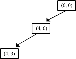
Figure 1.6: A Depth-First Search Tree
The search procedure we have just described is also called
depth-first search. The following algorithm describes this precisely.
Algorithm:
Depth-First Search
- If the initial state is a goal state, quit and return success.
- Otherwise, do the following until success or failure is
signaled:
a)
Generate a successor, F, of the
initial state. If there are no more successors, signal failure.
b)
Call Depth-First Search with E
as the initial state.
c)
If success is returned, signal
success. Otherwise continue in this loop.
Figure 1.6 shows a snapshot of a depth-first search for the water
jug problem. A comparison of these two simple methods produces the following
observations.
Advantages of Depth-First Search
- Depth-first search requires less
memory since only the nodes on the current path are stored. This contrasts
with breadth-first search, where all of the tree that has so far been
generated must be stored.
- By chance (or if care is taken in
ordering the alternative successor states), depth-first search may find a
solution without examining much of the search space at all. This contrasts
with breadth-first search in which all parts of the tree must be examined
to level n before any nodes on level n + 1 can be examined. This is
particularly significant if many acceptable solutions exist. Depth-first
search can stop when one of them is found.
Advantages
of Breadth-First Search
Breadth-first
search will not get trapped exploring a blind alley. This contrasts with
depth-first searching, which may follow a single, unfruitful path for a very
long time, perhaps forever, before the path actually terminates in a state that
has no successors. This is a particular problem in depth-first search if there
are loops
1.2.9
Bidirectional Search
The object of a search procedure is to discover a path through a
problem space from an initial configuration to a goal State. While PROLOG only
searches from a goal state, there are actually two directions in which such a
search could proceed:
Ø
Forward, from the start states
Ø
Backward, from the goal states
The production system model of the search process provides an easy
way of viewing forward and backward reasoning as symmetric processes. Consider
the problem of solving a particular instance of the 8-puzzle. The rules to be
used for solving the puzzle can be written as shown in Figure 1.3. Using those
rules we could attempt to solve the puzzle shown in Figure 1.4 in one of two
ways:
Reason
forward from the initial states. Begin building a tree of move sequences that might be solutions by
starting with the initial configuration(s) at the root of the tree. Generate
the next level of the tree by finding all the rules whose left sides
match the root node and using their right sides to create the new
configurations. Generate the next level by taking each node generated at the
previous level and applying to it all of the rules whose left sides match it.
Continue until a configuration that matches the goal state is generated.

Square I empty and Square 2 contains tile n ®
Square 2 empty and Square 1 contains tile n
Square I empty and Square 4 contains tile n ®
Square 4 empty and Square 1 contains tile n
Square 2 empty and Square 1 contains tile n ®
Square I empty and Square 2 contains tile n
:
Figure
1.4: A Sample of the Rules for Solving the 8-Puzzle
Reason
backward from the goal states. Begin building a tree of move sequences that might be solutions by
starting with the goal configuration(s) at the root of the tree. Generate the
next level of the tree by finding all the rules whose right sides match
the root node. These are all the rules that, if only we could apply them, would
generate the state we want. Use the left sides of the rules to generate the
nodes at this second level of the tree. Generate the next level of the tree by
taking each node at the previous level and finding all the rules whose right
sides match it. Then use the corresponding left sides to generate the new
nodes. Continue until a node that matches the initial state is generated. This
method of reasoning backward from the desired final state is often called goal-directed
reasoning.
Notice that the same rules can be used both to reason forward from
the initial state and to reason backward from the goal state. To reason
forward, the left sides (the preconditions) are matched against the current
state and the right sides (the results) are used to generate new nodes until
the goal is reached. To reason backward, the right sides are matched against
the current node and the left sides are used to generate new nodes representing
new goal states to be achieved. This continues until one of these goal states
is matched by an initial state.
In the case of the 8-puzzle, it does not make much difference
whether we reason forward or backward; about the same number of paths will be
explored in either case But this is not always true. Depending on the topology
of the problem space, it may be significantly more efficient to search in one
direction rather than the other.
Four factors
influence the question of whether it is better to reason forward or backward:
Ø Are there more possible start states or goal states? We would like
to move from the smaller set of states to the larger (and thus easier to find)
set of states.
Ø In which direction is the branching factor (i.e., the average number
of nodes that can be reached directly from a single node) greater? We would
like to proceed in the direction with the lower branching factor.
Ø Will the program be asked to justify its reasoning process to a
user? If so, it is important to proceed in the direction that corresponds more
closely with the way the user will think.
Ø What kind of event is going to trigger a problem-solving episode? If
it is the arrival of a new fact, forward reasoning makes sense. If it is a
query to which a response is desired, backward reasoning is more natural.
A few examples make these issues clearer. It seems easier to drive
from an unfamiliar place home than from home to an unfamiliar place. Why is
this? The branching factor is roughly the same in both directions (unless
one-way streets are laid out very strangely). But for the purpose of finding
our way around, there are many more locations that count as being home than
there are locations that count as the unfamiliar target place. Any place from
which we know how to get home can be considered as equivalent to home. If we
can get to any such place, we can get home easily. But in order to find a route
from where we are to an unfamiliar place, we pretty much have to be already at
the unfamiliar place. So in going toward the unfamiliar place, we are aiming at
a much smaller target than in going home. This suggests that if our starting
position is home and our goal position is the unfamiliar place, we should plan
our route by reasoning backward from the unfamiliar place.
On the other hand, consider the problem of symbolic integration. The
problem space is the set of formulas, some of which contain integral
expressions. The start state is a particular formula containing some integral
expression. The desired goal state is a formula that is equivalent to the
initial one and that does not contain any integral expressions. So we begin
with a single easily identified start state and a huge number of possible goal
states. Thus to solve this problem, it is better to reason forward using the
rules for integration to try to generate an integral-free expression than to
start with arbitrary integral-free expressions, use the rules for
differentiation, and try to generate the particular integral we are trying to
solve. Again we want to head toward the largest target; this time that means
chaining forward.
These two examples have illustrated the importance of the relative
number of start states to goal states in determining the optimal direction in
which to search when the branching factor is approximately the same in both
directions. When the branching factor is not the same, however, it must also be
taken into account.
Consider again the problem of proving theorems in some particular
domain of mathematics. Our goal state is the particular theorem to be proved.
Our initial states are normally a small set of axioms. Neither of these sets is
significantly bigger than the other. But consider the branching factor in each
of the two directions. From a small set of axioms we can derive a very large
number of theorems. On the other hand, this large number of theorems must go
back to the small set of axioms. So the branching factor is significantly
greater going forward from the axioms to the theorems than it is going backward
from theorems to axioms. This suggests that it would be much better to reason
backward when trying to prove theorems. Mathematicians have long realized this,
as have the designers of theorem-proving programs.
The third factor that determines the direction in which search
should proceed is the need to generate coherent justifications of the reasoning
process as it proceeds. This is often crucial for the acceptance of programs
for the performance of very important tasks. For example, doctors are unwilling
to accept the advice of a diagnostic program that cannot explain its reasoning
to the doctors’ satisfaction. This issue was of concern to the designers of
MYCIN, a program that diagnoses infectious diseases. It reasons backward from
its goal of determining the cause of a patient’s illness. To do that, it uses
rules that tell it such things as “If the organism has the following set of
characteristics as determined by the lab results, then it is likely that it is
organism x. By reasoning backward using such rules, the program can answer
questions like “Why should I perf5rm that test you just asked for?”
with such answers as “Because it would help to determine whether organism x is
present.”
By describing the search process as the application of a set of
production rules, it is easy to describe the specific search algorithms without
reference to the direction of the search. We can also search both forward from
the start state and backward from the goal simultaneously until two paths meet
somewhere in between. This strategy is called bidirectional search. It seems appealing if the number of
nodes at each step grows exponentially with the number of steps that have been
taken. Empirical results suggest that for blind search, this divide-and-conquer
strategy is indeed effective. Unfortunately, other results suggest that for
informed, heuristic search it is much less likely to be so Figure 1.5 shows why
bidirectional search may be ineffective. The two searches may pass each other,
resulting in more work than it would have taken for one of them, on its own, to
have finished. However, if individual forward arid backward steps are performed
as specified by a program that has been carefully constructed to exploit each
in exactly those situations where it can be the most profitable, the results
can be more encouraging. In fact, many successful Al applications have been
written using a combination of forward and backward reasoning, and most AI
programming environments provide explicit support for such hybrid reasoning.
Although in principle the same set of rules can be used for both
forward and backward reasoning, in practice it has proved useful to define two
classes of rules, each of which encodes a particular kind of knowledge.
Ø Forward rules, which encode knowledge about how to respond to
certain input configurations.
Ø Backward rules, which encode knowledge about how to achieve
particular goals.
By separating rules into these two classes, we essentially add to
each rule an additional piece of information, namely how it should be used in
problem solving. In the next three sections, we describe in more detail the two
kinds of rule systems and how they can be combined.

Figure
1.5: A Bad Use of Heuristic Bidirectional Search
Backward-Chaining Rule Systems
Backward-chaining rule systems, of which PROLOG is an example, are good for goal-
directed problem
solving. For example, a query system would probably use backward chaining to
reason about and answer user questions.
In PROLOG, rules are
restricted to Horn clauses. This allows for rapid indexing because all of the
rules for deducing a given fact share the same rule head. Rules are matched
with the unification procedure. Unification tries to find a set of bindings for
variables to equate a (sub) goal with the head of some rule. Rules in a PROLOG program are matched in the order
itt which they appear.
Other backward-chaining systems allow for more complex rules. In MYCIN, for example, rules can be
augmented with probabilistic’ certainty factors to reflect the fact that some
rules are more reliable than others.
Forward-Chaining Rule Systems
Instead of being directed by goals, we sometimes want to be directed
by incoming data. For example, suppose you sense searing heat near your hand.
You are likely to jerk your hand away. While this could be construed as
goal-directed behavior, it is modeled more naturally by the recognize-act cycle
characteristic of forward-chaining rule systems. In forward-chaining systems,
left sides of rules are matched against the state description. Rules that match
dump their right-hand side assertions into the state, and the process repeats.
Matching is typically more complex for forward-chaining systems than
backward ones. For example, consider a rule that checks for some condition in
the state description and then adds an assertion. After the rule fires, its
conditions are probably still valid, so it could fire again immediately.
However, we will need some mechanism to prevent repeated firings, especially if
the state remains unchanged.
While simple matching and control strategies are possible, most
forward-chaining systems (e.g., OPS5) implement highly efficient matchers and
supply several mechanisms for preferring one rule over another.
Combining Forward and Backward Reasoning
Sometimes certain aspects of a problem are best handled via forward
chaining and other aspects by backward chaining. Consider a forward-chaining
medical diagnosis program. It might accept twenty or so facts about a patient’s
condition, then forward chain on those facts to try to deduce the nature and/or
cause of the disease. Now suppose that at some point, the left side of a rule
was nearly satisfied—say, nine
out of ten of its preconditions were met, It might be efficient to apply
backward reasoning to satisfy the tenth precondition in a directed manner,
rather than wait for forward chaining to supply the fact by accident. Or
perhaps the tenth condition requires further medical tests. In that case,
backward chaining can be used to query the user.
Whether it is possible to use the same rules for both forward-and
backward reasoning also depends on the form of the rules themselves. If both
left sides and right sides contain pure assertions, then forward chaining can
match assertions on the left side of a rule and add to the state description
the assertions on the right side. But if arbitrary procedures are allowed as
the right sides of rules, then the rules will not be reversible. Some production
languages allow only reversible rules; others do not. When irreversible rules
are used, then a commitment to the direction of the search must be made at the
time the rules are written. But, as we suggested above, this is often a useful
thing to do anyway because it allows the rule writer to add control knowledge
to the rules themselves.
No comments:
Post a Comment